Auto Insurance Risk Classification and Claim Prediction
Contents
Data Research at the level of data base and excluding first set of features
Data Profile and preliminary feature importance ordering
Gini coefficient for 8 train/test sizes
DW Data Model for Predicted Data and Models description
Pentaho SPOON ETL to predict and re-train the model
Introduction
The goal of the project is to build a dashboard to analyze how risky are policies and effective current rates.
The current state of the data does not allow easily accomplish even the first step - creating training and test data sets. So, the first objective is to research available data sources and add into the corporate Data Warehouse all needed data in a form available for further processing.
After the predictive model itself is ready I need a data model to keep the predictive model data and results in DW and build an ETL process to predict the results and re-train the model time to time .
It's only a schematic description to provide understanding of the environment and challenges:
. Production Transactional System: an XML-based data source. XMLs are physically stored in varchar type columns in MS SQL database tables.
. A regular process converts some XML data into relational tables in another MS SQL database. Historical reports are run from this database.
. ETL process loads data into the corporate DW.
Even available data in the relational form is a challenge for DW ETL because there are no unique keys (except policies and claims), valid foreign keys, last update dates and history.
DW original data model and ETL process is a third-party product not fully customized for the company data and processes.
DW Data Model
Traditional DW approach is to create a slowly changing dimension (SCD) type 2 for entities changing over time. Vehicle's Estimated Annual Distance or Drivers MVR Status can be different in each term and it impacts rates. It works best with transactional based fact table where you can see what's changed in a risk attributes and how it impacts metrics. The dimension is directly joined to a fact table.

Figure 1 Policy transaction schema with subtype automobile from Ralph Kimball The Data Warehouse Toolkit 3rd edition
On the other hand, in ongoing monthly or yearly reports only a current state of a policy at the end of a month is taken into account. For historical reports only a last state of a policy term is taken into account.
Prediction data sets are more like historical reports. We need some point in time when we take the data. The last policy state or policy term state works for this purpose.
In a real word, the process is even more complex because it is not just one object (vehicle) which can be in different states but 2 independent objects - vehicle and driver. They can change their states independently.
Each of the objects has plenty (20+) attributes and combining them into one table does not make sense. Especially, taking into account we would like a similar approach for other line of business (Commercial Properties, Homeowners, Dwelling) where the level of details for insured items even more deep (200+ attributes).
Creating 2 traditional SCD dimensions type 2 for DIM_VEHICLE and DIM_DRIVER is not a big deal. There are few issues however in our source systems: missing unique entities IDs, change dates and historical information. Some of this missing info can be added into the source data base from XML original data source and adjusting current parsing procedure but it takes significant amount of research, resources and time. So, for now some surrogate data are used as unique entities ID's and change dates. We loss some information but it's acceptable as for now.
The other issue of the available source data is the place of the fields. Some vehicle attributes look not in proper place and the other should be combined. I would use a policy level instead. More work is required to investigate XML-based data source to get historical data in a proper format.
The dimensions are usually directly joined to fact tables to track the history of changes in risks. And this is the other issue - the data model in our DW is 4sightBI based and was designed without this level of details (insured items in SCD type 2). There is also no separation by line of business. We have just one set of FACT tables for all of them. E.g. all Auto and Homeowners transactions are in one table. In this way, one row in a fact table should have relation to DIM_VEHICLE and DIM_DRIVER and the other one to DIM_BUILDING.
It is not just a matter of adding new relations to Fact tables but also adjusting ETL. The ETL process is built in Pentaho Spoon in a way to support several different data base types (e.g. JavaScript based not T-SQL or PL/SQL procedures). Adjusting and testing this type of process is not easy and fast.
The good thing, however, there is a DIM_COVEREDRISK dimension (and references in FACT tables) in the original data model. It's a general table without specific to risk items attributes.
So, the solution is to reuse DIM_COVEREDRISK and join SCD type 2 DIM_VEHICLE and DIM_DRIVER not to the fact tables directly but rather to DIM_COVEREDRISK as a bridge table. The insured items dimensions from other line of business also can be joined to fact tables via DIM_COVEREDRISK in the same way. There are few type fields in the dimension and we can describe what exactly dimension is joined in a row.
To make life easier I added several more columns in DIM_COVERDRISK. It allows now to join a fact table row to an exact historical record in SCD2 item dimension or to the item version corresponding to the end of a specific term or policy.
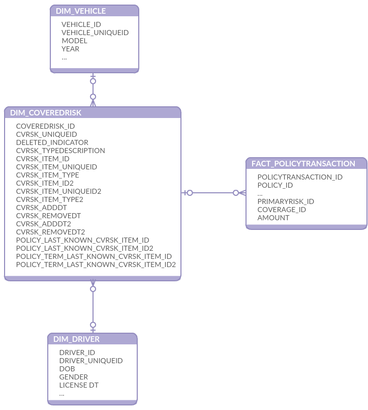
Figure 2 Extension for 4SightBI DW schema, DIM_VEHICLE and DIM_DRIVER SCD type2 joined via DIM_COVEREDRISK to FACT_POLICYTRANSACTION
Building Classification Model
While DW model is still under construction, I used both intermediate data source (a relation data base, but not DW star schema) and data available in DW. The process (set of SQLs) is very cumbersome.
Only unique vehicle and primary driver combinations from the last existing policy terms were used to create the train and test data set. It means there are no repeatable vehicle and driver pairs with different parameters (age) in the set even if they were insured for years.
HasClaim = 1 if there are one or more at fault claim for driver-vehicle combination. At fault claims for non-primary drivers were added into the data set to take into account all claims.
As expected there are only 5.5% of driver-vehicle combinations with claims. It's comparable with other datasets described in the open sources.
However, the dataset looks incomplete because non-primary drivers and age changes without claims are not taken into account.
The process to get all needed data is still quite complex and requires new structures in DW.
ToDo:
What happen if add in the data set all available policy terms because in the approach described above the age (driver, license, vehicle) is frozen? On the other hand, the samples will be dependable on each other.
Try to add in the data set non-primary drivers - vehicle combinations plus vehicles without drivers with all other drivers combinations
The claim rate may change to ~3%.
I am new in Insurance industry and know little what can impact claims. It is interesting to discover features on my own using machine learning and compare to what is used in a real word.
There are available articles about using machine learning in insurance but not a lot information or justification what features were actually used. So, I started working with all features related to vehicles and drivers I was able to find plus few calculated. At the end of the article I added the final list of features which do impact the model.
Due to the data relation issues GEO information (zip,city) were not added at the first stage. Though I do not believe it should impact at fault claims. There is a garage code in Vehicle data so let's see.
Several features were added into the list from an external source by VIN number. The idea was to check if there is something else which impact the claims but not in the company data. The other reason is to get more clean data. Some high cardinality categorical features in the company data are not standardized and have even more levels then needed (manufacturer and model).
External features:
. engine
. height
. length
. width
. make (manufacturer)
. model
. model year
. model score
Few web-scrappers were created to pull free available information by vehicle number
http://www.carinsurance.com/calculators/average-car-insurance-rates.aspx
The age features (DriverAge, VehicleAge, HaveLicenseAge, MVRStatusAge, etc) were calculated based on date type fields and the last known transaction date for vehicle-driver pair or loss date.
Totally there were 60 features in the initial list. Most of them are categorical with several high cardinality columns.
Here is the initial list of features I started with
Data Research at the level of data base and excluding first set of features
When the data sources are known and the plan of data selection is set we can review the available features if it even makes sense to include them into the data set for further investigation. It's a simple step and it's easy to perform while the data is in a data base using SQL.
What I verified at this step:
1. Total number of records.
2. Number of records in each class.
3. What's the percent of the values are empty(Null) or have default values if they are from a DW. There are maybe attributes recently added to the system and not yet populated for a representative amount of records. The other reason of high level empty values is using customization in out of the box systems with a lot default attributes not used in the company. Few records maybe populated by mistake/training or in first customized versions.
Migration data from retired systems to a new one also may create not consistent set of features. If percent is relatively low but a column is no longer used it does not make sense to rely on the feature.
If the percent is very high it does not make sense to add the feature into the final data set.
4. % of empty(Null) or default values per class. If one class has high percent and the other one is almost always empty(default) it also does not make sense to include it into the model. It may be an issue in the data collection.
5. Number of unique values per each feature. If there is just one value it does not make sense to continue research of this feature.
The results can be found in this Excel workbook.
Data set characteristics
1. It consists from unique per company data vehicle-driver pairs
2. Target variable is HasClaim:
a. 1 if there were one or more claims in this particular vehicle-driver pair (Minority class).
b. 0 if no claims were observed for the whole life of the policy (Majority class).
3. 50+ features.
4. Most of the features are categorical (text).
5. Several of them are high cardinality categorical features (100+ levels).
6. Highly unbalanced (minority class is only 5.5%)
7. There are no null values, instead there are default values (the data were selected form a DW)
8. The features are populated at least at 70% level. E.g. no one feature has more then 30% default values.
Data Preparation
Python was used at this stage of project.
Most of the data in the data set are categorical. To feed them into a machine learning algorithm in Python it should be converted into numerical.
Traditionally one-hot encoding is used to prevent the model to assume ordinal relationship between encoded integer values for each categorical input variable.
According to the discussion and my own several tests it looks like one-hot encoding is not needed for tree-based algorithms.
I applied Pandas Categorical codes for each categorical feature adding "_encd" to the name and save the results in a file to be used in further research.
See this file for details.
Some statistical research (see below) can not work with high cardinality columns. I tried not just clustering (Kmeans and Hclust) to limit the number of levels but also targeting encoding using this code. You can find more details regarding the method in Feature Engineering section below.
Data Profile and preliminary feature importance ordering
At this stage I used R to get general information regarding each feature: type, number of 0, null (in this case not applicable since I used DW data where all nulls are replaced with a default value but can reveal some issues in data joining and selection), infinity and unique values, samples of values, Median, Mean, 3rd Qu, Max for numerical or levels for categorical.
I rejected some features at this step where are two levels but one of them have only very few records.
Features correlation is also calculated and visualized as a part of the data profile.
I calculated Shapiro test to test normality of few numerical values as a part of data profiling but in this case, it is optional because XGB, which I was going to use later, does not need normalization for better results.
The following methods were used to build base set of features and start feature importance research:
o Statistical (R):
ChiSq test to test significance of the relation between categorical features and target and Cramer V test to measure the association.
Wilcox test to test dependence numerical features with the target.
o Information Values (R) Though, if a sample size is small, the metric is not very reliable
o Boruta Features Selection with Random Forest to rank features (Python).
o XGB Features Importance with algorithm default parameters and random under sampling for balancing (Python).
Principal Components Analysis was also done, but it does not make sense in this case because too many information is lost.
The output of this step is few consolidated tables. I manually set feature importance based on the results of all methods.
These features are most important according to the preliminary research:
|
Feature |
Importance |
|
Driver Age |
1 |
|
Class |
1 |
|
Vehicle Age |
1 |
|
MVR Status Age |
1 |
|
MVR Status |
1 |
|
Estimated Annual Distance |
2 |
|
Occupation |
2 |
|
Driver Number |
2 |
|
Vehicle Body Type |
2 |
|
Good Driver |
2 |
|
Odometr Reading |
2 |
|
Marital Status |
2 |
|
Mature Driver |
2 |
|
Vehicle Number |
2 |
|
Carpool |
2 |
|
Driver Status |
2 |
|
ISO Rating Value |
2 |
|
Accident Prevention Course |
2 |
|
Daylight Driving |
2 |
|
Driver Training Course |
2 |
The rest are noise.
XGB
Gradient Boosting (GB) is a relatively new method for building insurance loss cost models. It's widely used in recent machine learning competitions. There are several advantages to comparing to the traditional Generalized Linear Models and other machine learning algorithms.
. GB works very well with the large number of categorical features. It requires relatively less data preprocessing and knows how to handle missing and imbalance data.
. We do have complex non-linear dependencies in the data and GB is a better choice then methods based on linear algorithms (GLM).
. Comparing to other non-linear methods like neutral networks it does not require millions of samples to train.
. It's a "white-box" approach and provides interpretable results via plots of features importance, partial dependencies and used decision trees.
There are several algorithms based on gradient boosting. XGB is faster and can be more accurate then Adaboost. LightGB has the same performance but works better with bigger data sets. In Kaggle competitions often all of them are used in an ensemble (ToDo later).
The model stacking (including GLM based models) reduces variance and provides better generalizability.
For the first step I used XGB alone.
I used 5000 trees (estimators) and 100 early stopping round for training.
I did not tune these parameters just selected high number of estimators and reasonable number of early stopping round to keep the model from overfitting.
ToDo test if less number of trees get the same result
Stratified fold
To make sure the data are generalized well and maximaze the usage of the information available in the training data I applied StratifiedKFold from sklearn to select a model. This method preserves the percentage of samples in each class. This is especially important in the case of highly imbalanced data set.
The common practice is to use 10-fold stratified cross-validation to get lower bias and variance.
Data Balancing
The dataset is highly unbalanced. There are only 5.5% of positive samples (have claims). A classification algorithm will tend to favor the class with the largest proportion of observations (e.g. samples without claims). We are interested in the samples with claims, minority class.
In my first experiments I used Random Under sampling to remove majority of no claims samples from the training data set. (See code to test different ratios.)
Later I started use scale_pos_weight XGB parameter. The best value is 0.3. This approach provides a higher metric value.
See code and the results. I applied the same approach described below for models evaluation. A csv file with model names and different scale_pos_weight values or Random Under sampling ratios was created. The code reads the file, builds models and compare results.
XGB Parameters
I used a brute force to tune XGB parameters: bayesian global optimization with gaussian processes.
There is implementation in Python for XGB parameters tuning
A few local maximum were found with the same metric values. I selected a set with less overfitting.
Traditional methods like GridSearchCV did not find an optimal combination.
Several modules were created to test different parameters sets (BayesianOptimization). A notebook was created to test the approach, then it's converted in a python program code which was run in a background mode.
The code produces an output in a file to monitor the progress (and stop if no progress anymore).
The output was stored in a file to analyze.
Models Evaluation
Imbalance data set is one of the most challenging problem. That's why the right model evaluation method is a main research issue. Traditional metrics (accuracy, sensitivity, specificity, precision) lead to a biased classification when the classes are not equally distributed.
In my model evaluation process I used the area under the ROC curve (Area under curve, AUC) and Gini coefficient.
AUC is equivalent to the probability that the classifier will rank randomly chosen positive sample higher than a randomly chosen negative sample. AUC value varies between 0.5 (random guessing) and 1. For at fault claim prediction task it's usually 0.6-0.8 (fair to good performance).
The other metric used in imbalance data classification is a chance-standardize variant of the AUC is Gini coefficient. It's related to AUC in this way:
G = 2AUC-1
Gini coefficient values are between 0 and 1 (complete separation between the 2 distribution).
Let's say G's are metric values obtained from the model on different train/test sizes. They are random variables, normally distributed.
To compare one model performance to an other I used two-tailed paired t test. The test asks the question: is the Gini coefficient of the two system different
. Null hypothesis: the 2 models have the same Gini coefficient
. Alternate hypothesis: one of the model has a different Gini coefficient
Paired t-test is used to calculate probability p that mean of G's would arise from null hypothesis
If p is sufficiently small (typically < 0.05) then reject the null hypothesis.
To research models based on different feature sets I did not create the sets dynamically. Instead, I described a model in an Excel spreadsheet where each line is a model and a column is a feature name (original or engineered). The spreadsheet is converted in an csv file and used in the code. The code reads the model definition from the file and run them one by one on 8 train/test sizes to calculate the metrics. Each model is compared to the first one described in the file (BaseModel) to get probability from t test. Based on the p value each model is categorized in one of the 3 groups: 1 - no changes, statistically the same as the BaseModel, 2 - significantly better then the BaseModel and 3 - significantly worse then the BaseModel.
The results (models metrics values, p and t values from t-test, group) are saved in an other csv file after each model run and can be reviewed while the main code is still running.
At the end, the file with results are saved together with model descriptions to simplify analyzing and historical references.
In this Excel workbook you can review the model descriptions tabs (they are saved as csv files and used in the code) and the output results. See All Individual Features tab as an example of a models tab and All Individual Features Results tab with the output.
Several Python notebooks and programs were created to read the model descriptions from csv files, apply some feature engineering if needed and output the comparison between the models. The notebooks were used to test the approach and then converted to a code and run in a background mode. You can find the links specific for each step below. Monitor notebook was used to review already analyzed models results from a program running in the background. The other Monitor (Models Results Visualization) notebook builds charts to compare overfitting between the models.
Feature Importance
Based on the information I gathered on Data Profile step I selected few features which are important according to all methods I applied for the initial research (base set marked as group 1 in the table above).
Next, I added other features one by one alone to the base set and compare results to the base set result.
Most of them are just noisy features and did not improve the result at all. If there is a positive change in the metric it is not statistically significant.
Some of the features (like Relationship To Insured) even decreased the result statistically significantly.
To find this bad feature I used Lesion studies. To understand what contributes to a model I removed (lesioning) features from a model.
Here is the notebook used to compare a Base Model (base set of features) to other models with addition more or one features. See also the code with the same functionality.
The final 21 features were investigated in a more traditional way. I reviewed partial dependency of each feature according to XGB Feature Importance order starting from the less important.
Several features were rejected because if there is a dependency from a feature it is not dependency on the feature value but rather how this information is collected in the original system.
Let's say there are 3 feature values: "Yes", "No" and "Unknown" (no value in the system). "Yes" and "No" have approximately the same probability of having claim and only "Unknown" is different. It looks like this information is collected specifically for drivers with claims. If it's a new driver in the system we can not predict using this feature.
External Features
There are several features describing vehicle parameters added from public data sources by VIN number. Since they are not easy available I review their performance in a separate step.
Only 2 of them are really important: extranal_length and external_width
The rest does not change the model performance statistically significant.
Feature Engineering
Simple Calculation is the way to improve mostly numerical features output. Though I tried encoded values of categorical features.
Frequency and Targeting Encoding is the way to deal with categorical features. No one high cardinality categorical feature was recognized as useful at Feature Importance step. I added these methods to the research with a thought to improve the high cardinality features performance.
The model descriptions and results are in Feature Engineering Workbook.xlsx.
Simple Calculation
At this step I investigated if there is any positive impact if I will use sum or difference or multiplication two or more features.
In the Models spreadsheet I added one more column (Formula) to keep the expression to investigate. The code builds the dynamic feature on a fly based on the column and compare a model with the engineered feature to a Base Model.
I did not find any visible improvement except 2 cases:
1. If features are strong by themselves, the combination is also strong but not statistically significant. It does not make sense to spend resources on transformation if we can include in the final model raw features and have the same improvement
2. [Driver Age] - [Age when Driver obtained the License] e.g. Driver License Age works much better then just [Age when Driver obtained the License]
Here is the notebook and code to apply this type of engineering.
Frequency Encoding
The idea of this method is to replace categorical feature values with numbers how frequently they are appeared in the training set.
I compared each encoded categorical feature to a base set of numerical features only to see if there is a better model performance then adding raw categorical feature. E.g. I have 2 sets of models where BaseModel is the same, only numerical features, and the rest are raw categorical in one set and encoded in the other set.
There is no significant improvement in any encoded categorical feature. Few features are better in the encoded form comparing to a base set of numerical features only but the effect disappeared when the encoded feature is added into the full model (other categorical features present).
Interesting fact regarding 2 high cardinality features:
. Manufacturer is an original feature from the system. The content is inconsistent. Several acronyms and similar words can be used for the same manufacturer: Toyota, TYTA, etc
. External_make is a feature found by VIN number in a public database. The names are standardized, e.g.it's always Toyota
Performance of the both features is low without encoding. It's much better with frequency encoding. But performance of External_Make, standardized feature, is higher then Manufacturer.
|
Feature |
Mean (Gini Coefficient) |
Comment |
|
Manufacturer |
0.315 |
Raw value from the system |
|
Manufacturer |
0.319 |
Frequency encoded |
|
external_make |
0.315 |
External feature - Manufacturer value found by VIN number from a public database |
|
external_make |
0.322 |
Frequency encoded |
The notebook and code for frequency encoding.
Targeting Encoding
The basic idea of the encoding is to replace categorical values with an estimate of the probability of positive target (HasClaim=1) using Bayesian approach. Target encoding is done according to the paper by Daniele Micci-Barreca.
Since the target attribute is involved in the encoding it's important to make sure the model is not overfitted. E.g. only training data are involved into the process. For the same purpose noise is added to the data. It's decrease the output metric but prevent overfitting.
The model spreadsheet a little bit more complex because it includes 3 more columns for each feature: feature name itself, min_samples_leaf, smoothing and noise_level. These 3 additional descriptors are used as parameters into target encoding function. -1 in all 3 of them means do not apply target encoding for this feature.
In my previous experiments I did not find any impact of min_samples_leaf and smoothing. These set of tests investigates only a change in noise_level.
As in frequency encoding step I compared performance of an targeting encoded feature to a base set of numerical features and raw feature performance.
In addition, I investigated if there is any value in binning targeting encoded features. E.g. after the feature encoded, the full range of values is separated to 10 bins and instead of an encoded value, a corresponded bin is used in a model.
Targeting encoding does not improve the model performance. In some cases the result even worse then without encoding.
Binned targeting encoding has even worse result.
Manufacturer performance is improved comparing to a model without encoding but less then in targeting encoding.
No change in external_make feature performance with the use of targeting encoding.
There is no sense to use targeting encoding to improve high cardinality features performance in this data set.
. Targeting Encoding notebook and code
. Targeting Encoding with Binning notebook and code
Classification Model
There are 2 final models were created. Both have the same parameters but different feature sets. The Extended model includes 2 additional external parameters: vehicle length and width.
XGB Parameters
|
Parameter |
Value |
|
objective |
binary:logistic |
|
scale_pos_weight |
0.3 |
|
colsample_bytree |
0.9 |
|
eta |
0.01 |
|
max_depth |
4 |
|
colsample_bylevel |
0.2 |
The rest are default
Features
|
Base |
Extended |
|
classcd |
classcd |
|
driverage |
driverage |
|
driverage-havelicenseage |
driverage-havelicenseage |
|
vehicleage |
vehicleage |
|
estimatedannualdistance |
external_length_in |
|
ratingvalue |
estimatedannualdistance |
|
vehbodytypecd |
ratingvalue |
|
mvrstatusage |
external_width_in |
|
mvrstatus |
mvrstatusage |
|
drivernumber |
mvrstatus |
|
vehnumber |
drivernumber |
|
gooddriverind |
vehbodytypecd |
|
acci_last_infractionage |
vehnumber |
|
maritalstatuscd |
gooddriverind |
|
carpoolind |
acci_last_infractionage |
|
gendercd |
maritalstatuscd |
|
carpoolind |
|
|
gendercd |
Classification Results
Gini coefficient for 8 train/test sizes
|
Model |
Base |
Extended |
|
S0.45 |
0.409827 |
0.413367 |
|
S0.4 |
0.416889 |
0.419341 |
|
S0.35 |
0.418909 |
0.420991 |
|
S0.3 |
0.418788 |
0.421717 |
|
S0.25 |
0.419003 |
0.420827 |
|
S0.2 |
0.421668 |
0.424555 |
|
S0.15 |
0.419313 |
0.420508 |
|
S0.1 |
0.416097 |
0.42026 |
|
Mean |
0.417562 |
0.420196 |
|
t-pvalue |
0.138648 |
|
|
t-statistic |
-1.57038 |
|
|
Group |
1 |
In test on 8 train/test sizes Extended model has a little bit higher result but statistically not significantly higher then Base model.
Both models have a similar dependency train and test results on test size. The more training data the close lines to each other.
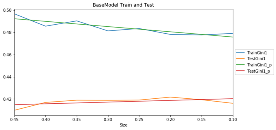
Figure 3 Base Model Train and Test results
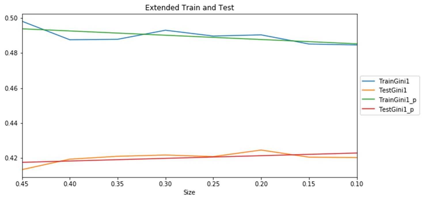
Figure 4 Extended Model Train and Test results
The result below is a random in some sense but can explain what's behind the metric we received.
To prepare data and charts below I used code from this folder.
80/20 % Train/Test results
|
Model |
Base |
Extended |
|
Test Gini |
0.420893 |
0.423917 |
|
Test ROC_AUC |
0.710447 |
0.711958 |
ROC Curve
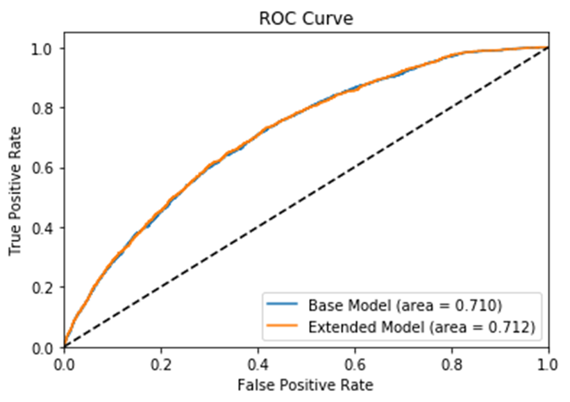
Figure 5 Base and Extended Models ROC Curves
Confusion Matrix
Base Model
|
True Positive |
930 |
False Positive |
9727 |
|
False Negative |
420 |
True Negative |
15498 |
Extended Model
|
True Positive |
924 |
False Positive |
9552 |
|
False Negative |
426 |
True Negative |
15673 |
Confidential interval
|
Number of samples (n) |
26575 |
|
for 95% confidence Zn |
1.96 |
|
Model |
Base |
Extended |
|
Number of errors: |
10147 |
9978 |
|
Error |
0.381825 |
0.375466 |
|
Confidence Interval |
0.00298 |
0.00297 |
Base Model: With approximately 85% probability, the true error 0.382 lies in the interval +/-0.003
Extended Model: With approximately 85% probability, the true error 0.375 lies in the interval +/-0.003
As you can see, the main improvement in Extended model is moving 200 vehicles from False Positive to True Negative due the vehicles dimensions.
Feature Importance
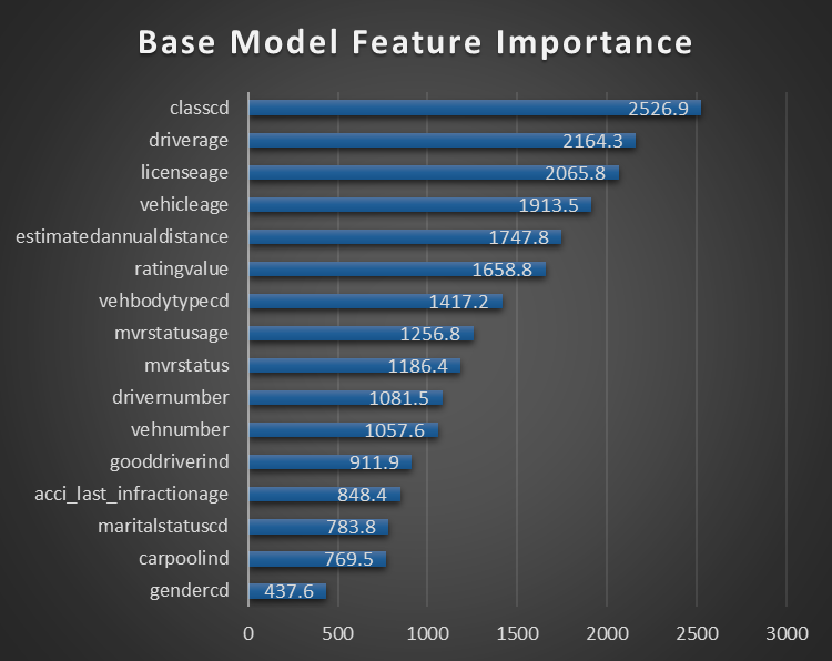
Figure 6 Base Model Feature Importance
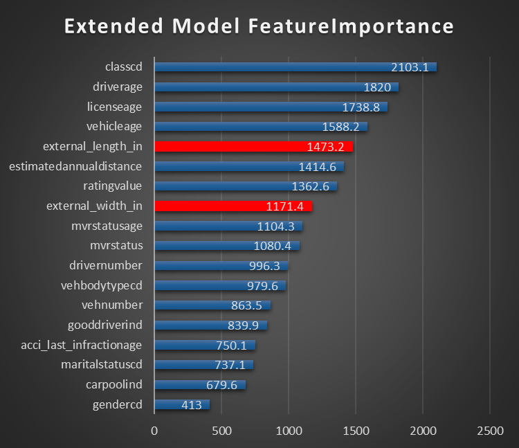
Figure 7 Extended Model Feature Importance
Age-related features are most important: driver age, driver license age, vehicle age, MVR Status Age. Class is also based on driver license age or vehicle age plus driver sender and marital status.
Gender is not very important and can be also removed.
Partial Dependency
Class is most important feature. It's based on several attributes of driver and vehicle together. It was added to Vehicle table in the relation data base but it rather belongs to something what's joined vehicle and driver together (policy or risk or applied rates or discounts table).
Apparently, class codes system is different in different states/products or rating. It is not easy to extract codes subsystems to show dependency. One of them is quite easy: There is a subsystem based on gender, marital status and driver license age. NNM(S)M(F) where NN is the driver license age, M is married, S is single and the second M is male, F is female.
Single Female have a higher probability of an accident starting from 19 years of driving. The cut-off driver license age for the rest of the population is 20 years.
Interesting, calculated driver license age, gender and vehicle age features without Class do not provide the same level of the metric. I think it's because there are missing values in the database and the date of obtaining of the driver license maybe the date of the current driver license, not the original.
|
|
|
|
Figure 8 Partial Dependencies for Single and Married Female and Male Figure 9 |
|
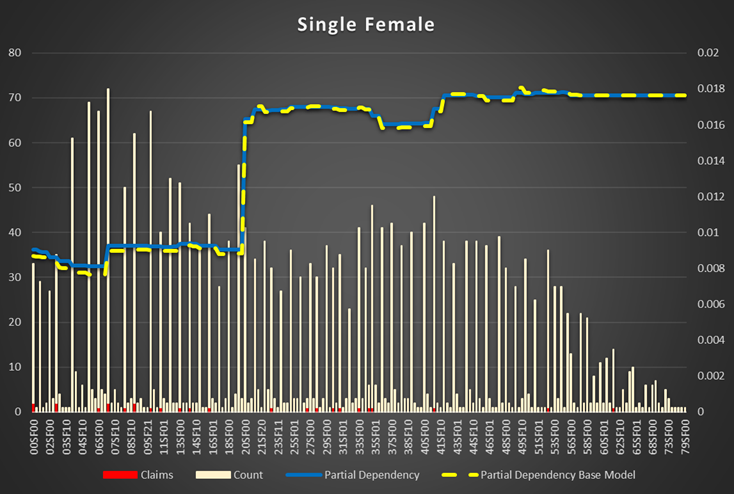
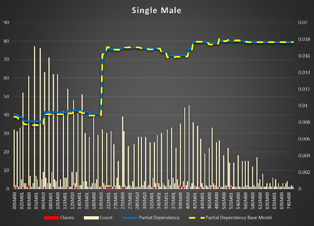
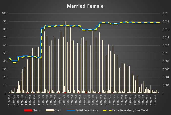
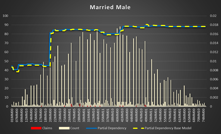
Figure 8 Partial Dependencies for Single and Married Female and Male
Driver Age is a second by importance feature. In fact, Class and Driver Age are almost the same by importance. Some models from the ensemble has Class as the first one, the others - driver Age.
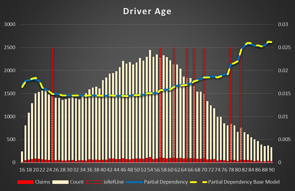
Figure 10 Partial Dependency for Driver Age
The risk of an accident is decreased from 20 to 25 years, then there is a big plateau between 25 and 57 years. It's gradually increased after 57 years and reach maximum at 81 years.
License Age (the difference between driver age and the age when the driver got the license).
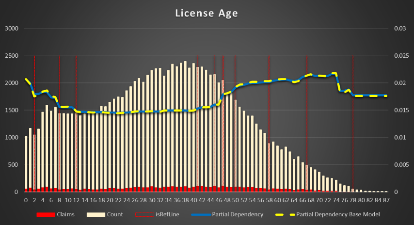
Figure 11 Partial Dependency for License Age
In general, it has approximately the same dependency as Driver Age. Decreased from 4 years till 12 years (20 - 28 years driver age), then a plateau till 48 years (64 years driver age) with maximum about 69 years (85 years driver age)
Vehicle Age. The plateau is till 9 years old and then the risk decreases. Apparently, the old vehicles are changed to newer and older if they are kept used less or more carefully.
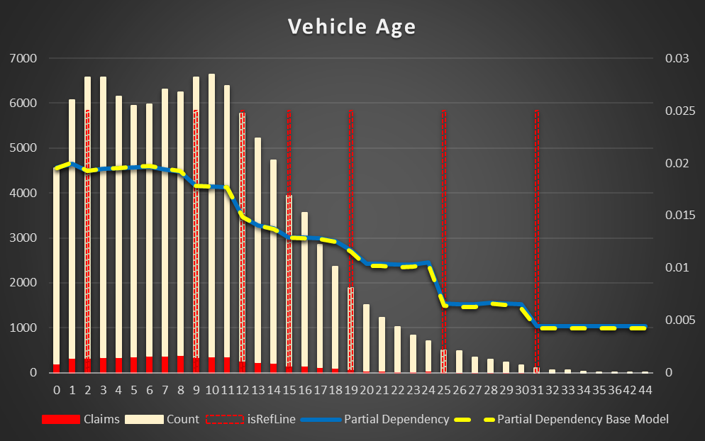
Figure 12 Partial Dependency for Vehicle Age
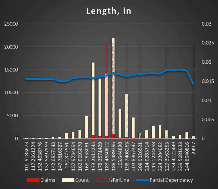
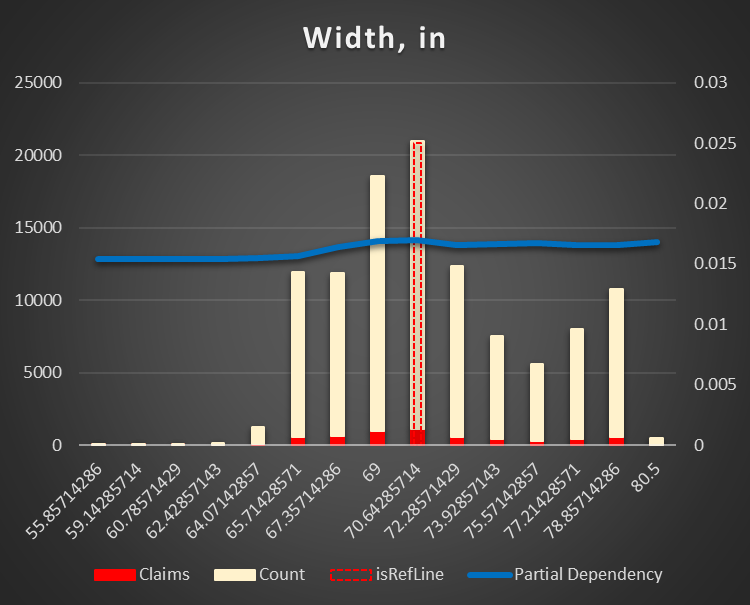
Vehicle dimensions (length and width in inches). The smaller (shorter and narrower) the vehicle, the less risk of an accident. Taking into account, the most of the accidents are related to parking it does make sense. It's much easy to park SMART then a truck or VAN.
|
Figure 13 Partial Dependency Vehicle Length,in |
Figure 14 Partial Dependency Vehicle Width,in |
Estimated Annual Distance is a simple one. The more you drive, the higher probability of an accident with a cut off point approximately 3,000 miles
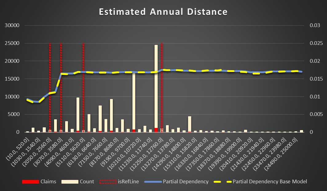
Figure 15 Partial Dependency Estimated Annual Distance
Rating Value. Vehicles with a higher rating have less chance to be in an accident. Though, the feature is not complete in the data. Looks like it's spread by few separated fields in the intermediate data base and not populated correctly in each run of the conversion from XML to a relation structure.
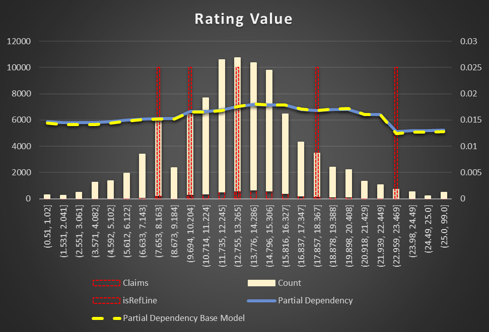
Figure 16 Partial Dependency ISO Rating
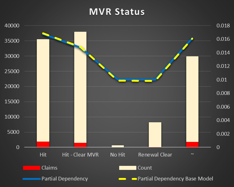
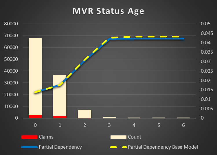
MVR Status and Age. The chance of an accident is lower just after a hit in terms of status and age. The more time after an accident the higher possibility of a new one. And I already mentioned the fact, the age importance is stronger, then the status.
|
Figure 17 Partial Dependency MVR Status |
Figure 18 Partial Dependency MVR Status Age |
Driver and Vehicle Numbers. Not clear if the numbers are related to real life use of the vehicles or it's just numbers used in documentation. The higher the number the higher accident risk.
Vehicle Body Type. The original feature has many levels due to non- standardized data. There is the same dependency as in the vehicle dimensions. The smaller the vehicle, the less chance of an accident. VANs, pickups, wagons have higher risk then sedans and coupes.
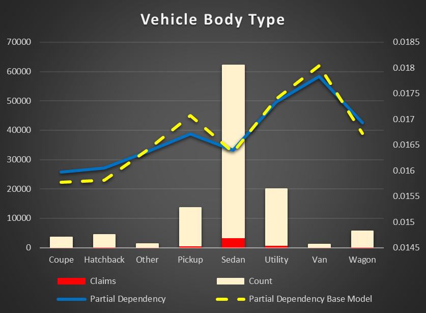
Figure 19 Partial Dependency Vehicle Body Type
Good Driver Flag(Discount) Most of the drivers are good, but it does not mean they have less risk of accidents. In fact, good drivers have a higher risk. Super drivers indeed have less chance of accidents.
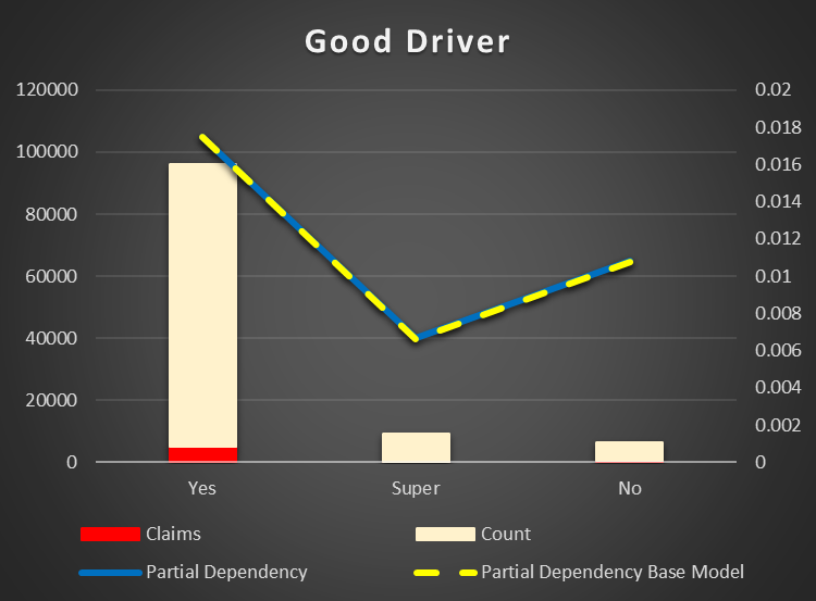
Figure 20 Partial Dependency Good Driver
Accident Last Infraction Age. There is the same dependency as with MVR Status and Age. The older a previous accident the higher chance of a new one. Interesting enough, Accident Points feature is not important to impact the result.
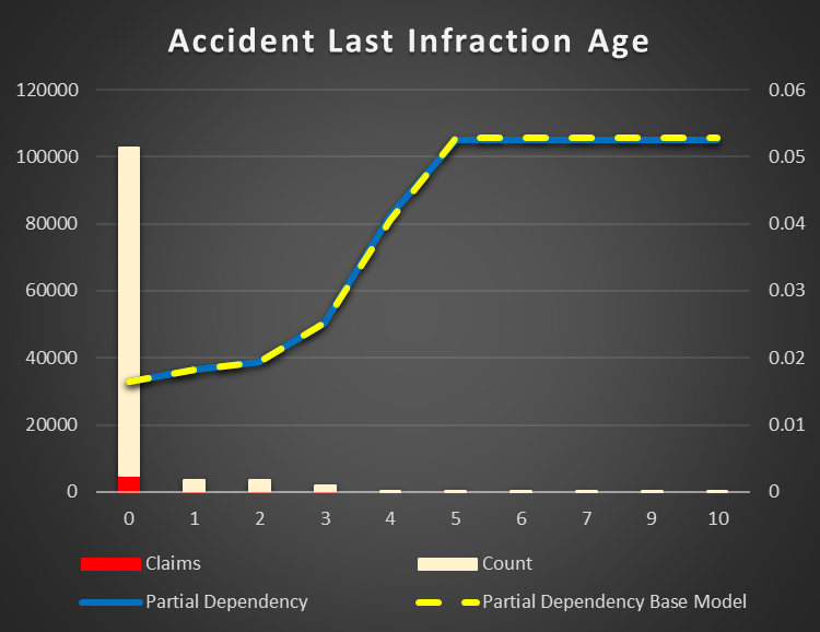
Figure 21 Partial Dependency Accident Last Infraction Age
Marital Status. Single persons have higher chance to cause an accident. It maybe related to the fact there are more single between youth and elderly.

Figure 22 Partial Dependency Marital Status
Carpool Flag (Discount). There are less accidents if drivers are carpool. It's naturally to carpool only if you are really a good driver. On the other hand, there are very few Yes in the data. The result maybe biased by the data collection. Anyway, it is not high important feature.
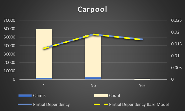
Figure 23 Partial Dependency Carpool Flag (Discount)
Gender can be excluded from the model. It does not make a lot of difference. Just interesting to notice, female have a higher risk of an accident then male.
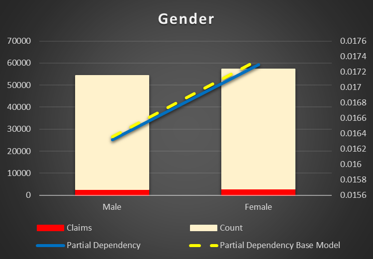
Figure 24 Partial Dependency of Gender
Regression Model (loss cost)
DW Data Model for Predicted Data and Models description
Pentaho SPOON ETL to predict and re-train the model
Dashboards
Summary
This is a multistage project.
At first stage the data sources were researched and the design of a DW data model with the risks items was created. While the work on DW ETL to include risks items data is still in progress, the data set for a machine learning model was built from an intermediaterelation dattabse data source and partially from DW what's already available. The SQL is quite cumbersome and does not allow to include all needed features.
Base and Extended classification machine learning models were created using XGB. The set of available in the system features was investigated to explain how they impact the risk of At Fault claim. Two additional features were discovered (vehicle length and width) to improve the prediction result.