Water Risk Scores Exploratory Data Analysis
Contents
Histogram
and claims partial dependency
Losses
mean plot with error bars
Histogram
and claims partial dependency
Losses
mean plot with error bars
Histogram
and claims partial dependency
Losses
mean plot with error bars
Histogram
and claims partial dependency
Losses
mean plot with error bars
Histogram
and claims partial dependency
Losses
mean plot with error bars
Histogram
and claims partial dependency
Losses
mean plot with error bars
Histogram
and claims partial dependency
Losses
mean plot with error bars
Introduction
All scores
are provided at the Census Block level. WaterRisk
Frequency reflects the relative liklihood of a
non-weather-water related loss, relative to the US. WaterRisk
Severity reflects the relative magnitude of a non-weather-water related loss,
relative to the US. WaterRisk 3.0 Total is the
combination of the Frequency Score and the Severity Score for that location and
reflects the relative risk of a non-weather-water loss at that location. Factor
Ratings are qualitative indications of the kinds of causes we would expect in
these locations. These are not quantitative, but are
provided for an underwriter to have a basis for discussion with an agent or
policy holder as to the kinds of causes that might be found, underlying the
score that is assigned.
R and Python code and output:
-
EDA.0.
Classification - Preparing Dataset for Frequency Feature Importance
-
EDA.1.
Feature Importance from XGB Classification
-
EDA.2.
Severity - Preparing Dataset for Gamma Distribution Feature Importance
-
EDA.3.
Severity - Feature Importance from XGB Gamma Distribution
-
EDA.4.
Severity - Preparing Dataset for Normal Distribution Feature Importance
-
EDA.5.
Severity - Feature Importance from XGB Regression
-
EDA.7
Frequency - Visualization_Final
- EDA.8 Severity - Visualization
Frequency
The cross_plot shows how the input
variable is correlated with the target variable, getting the likelihood rates
for each input's bin/bucket
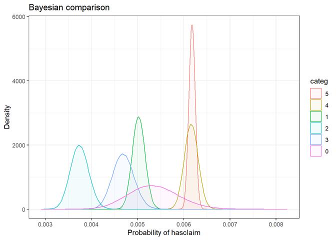
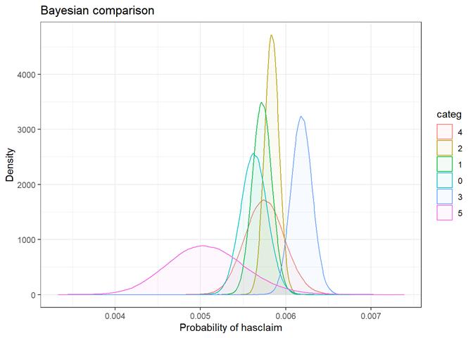
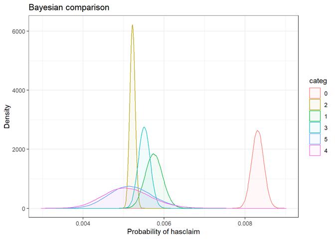
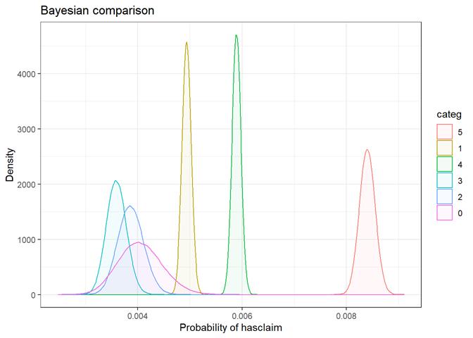
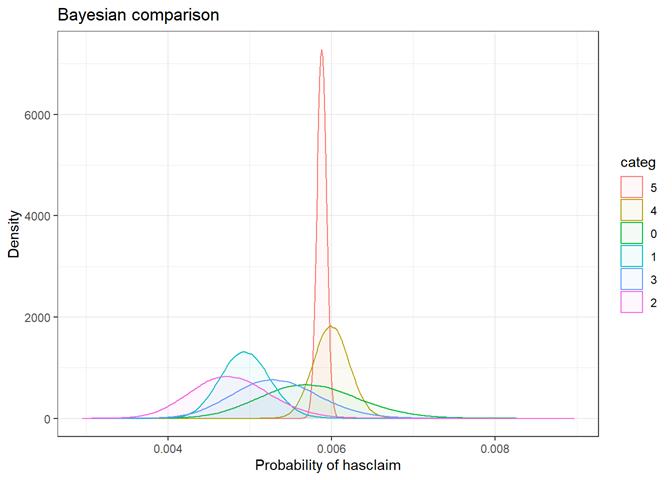
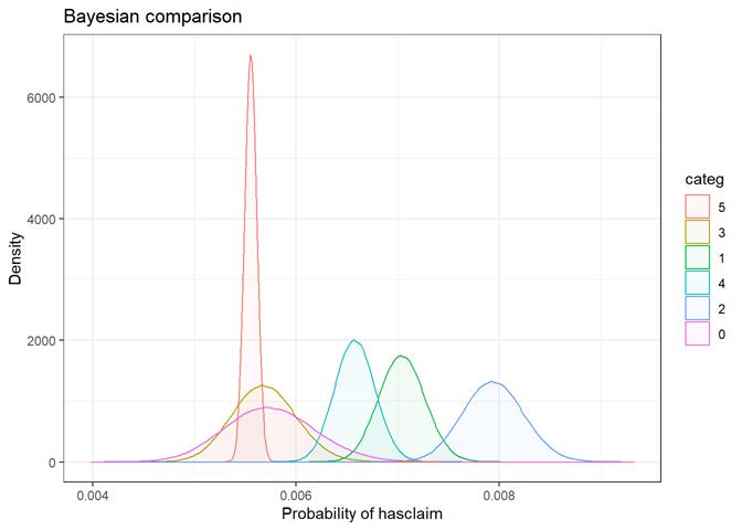
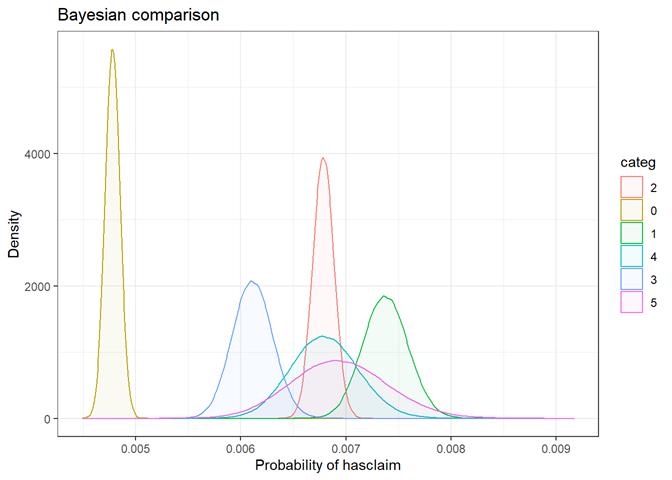
The bayesian_plot shows how the input variable is correlated with the target variable, comparing with a bayesian approach the posterior conversion rate to the target variable. It`s useful to compare categorical values, which have no intrinsic ordering (not ordered).
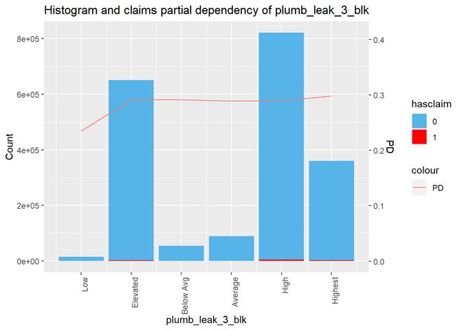
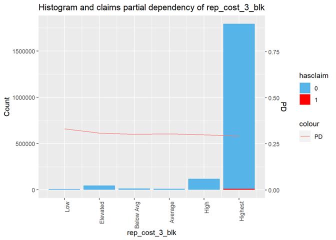
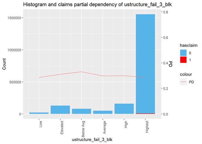
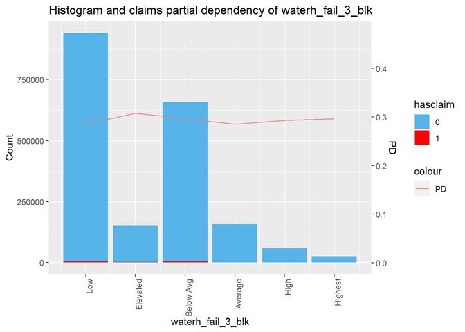
The third type of plots is the combination a bar-plot with the number of observations in each group, filled with the number of observations with claims and partial dependency plot from XGBoost classification.
For continuous attribute the most informative is a box-plot and partial dependency plot. The other plots are used to check if the distribution is close to the normal.
Since there are very few exposures with more then 1 claim, in this stage of analysis I use hasclaim (0/1 or No/Yes) attribute as the target instead of the real number of claims per exposure.
Severity
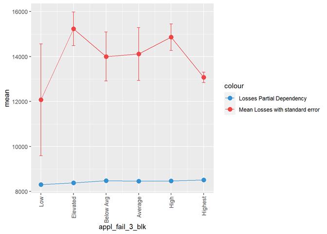
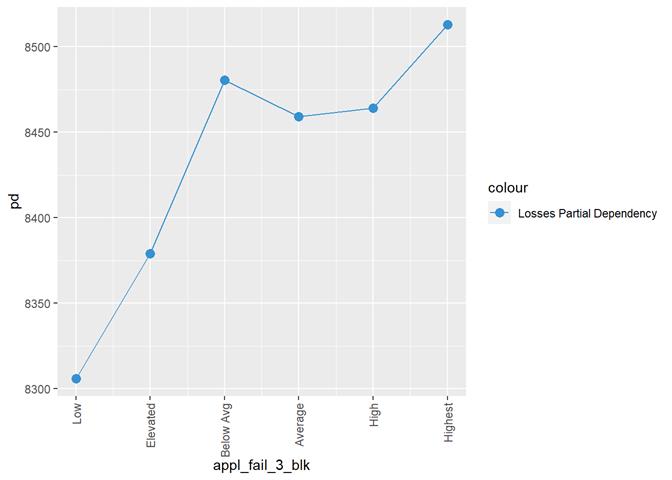
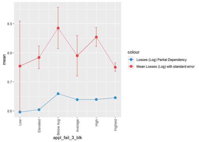
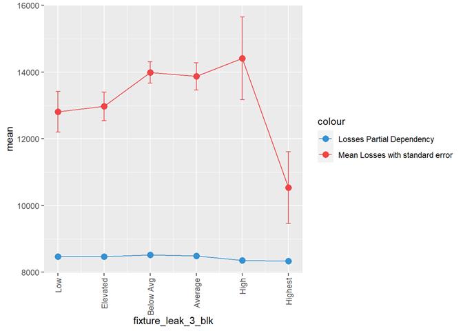
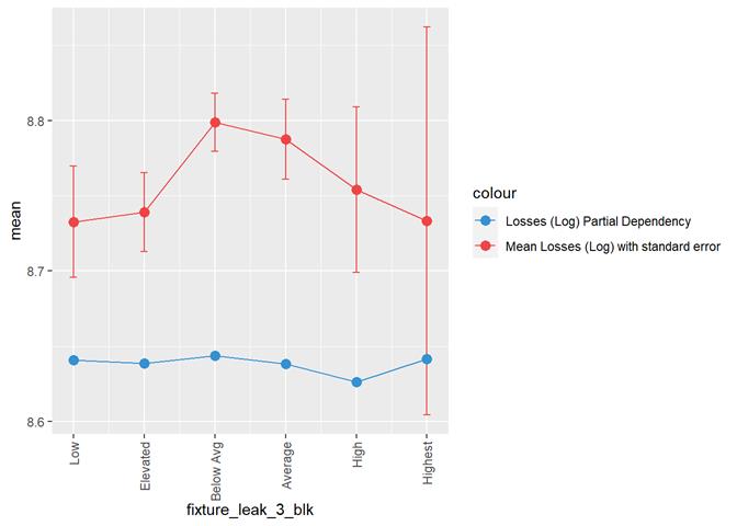
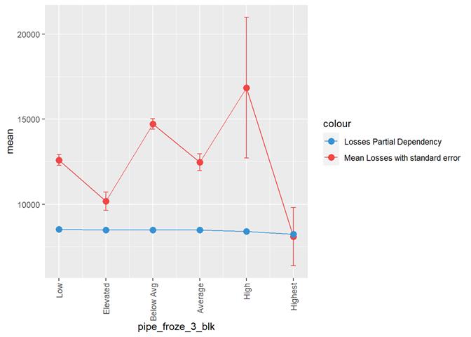
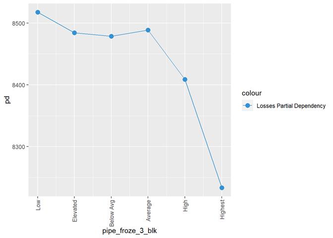
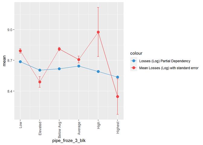
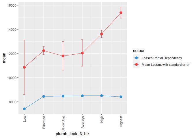
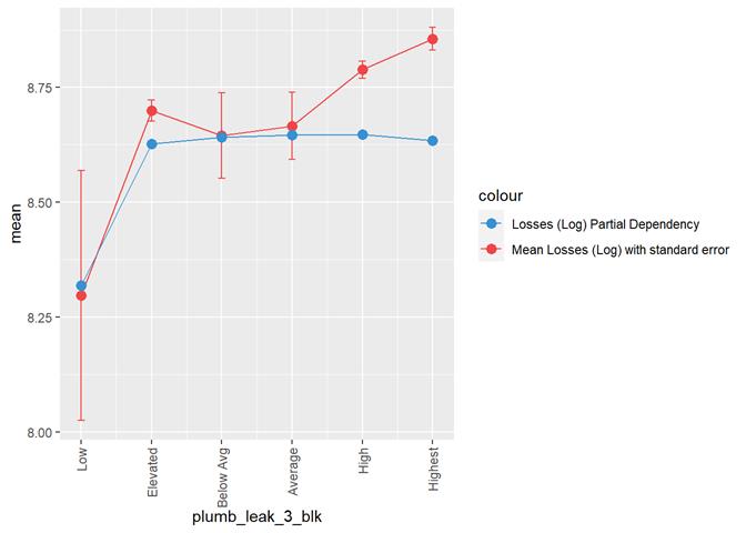
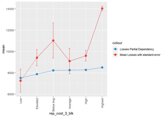
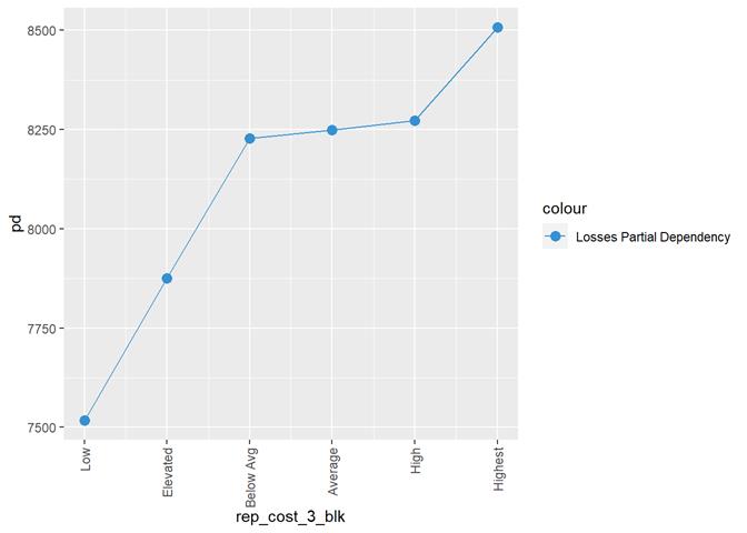
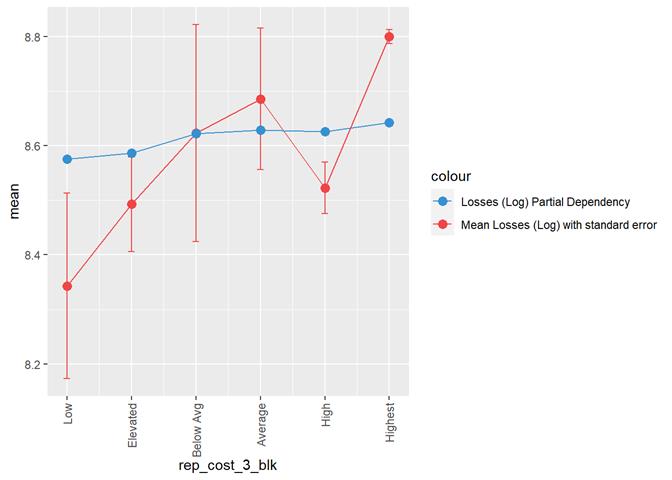
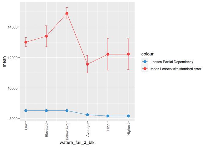
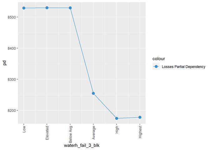
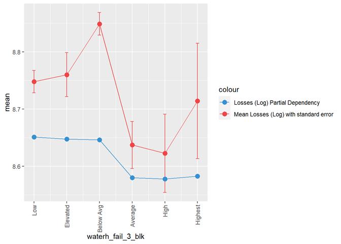
A popular method for comparing groups on a continuous variable is the mean plot with error bars. Error bars represents standard error in this section. The second plot is partial dependence plot from Gamma XGBoost regression or XGBoost regression (normal distribution for log of losses - cova_il_nc_water)
Scores
Th only interest for the further analysis is water_risk_3_blk for frequency and water_risk_sev_3_blk and, and maybe, rep_cost_3_blk for severity.
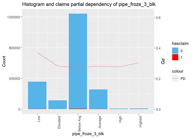
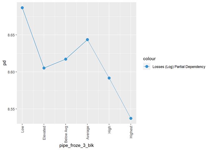
Pipe_froze_3_blk shows a dependency with the number of claims but not useful for analysis. Low score has the highest rate of claims, which maybe, makes sense for California, but not for the models.
The categorical scores were encoded to be used in some analysis methods:
|
Highest |
5 |
|
High |
4 |
|
Average |
3 |
|
Below Avg |
2 |
|
Elevated |
1 |
|
Low |
0 |
water_risk_3_blk
Non-weather Water Damage Loss Index relative to Nation (0 to 5000: 100=average, 50=0.5x average, 500=5x average)
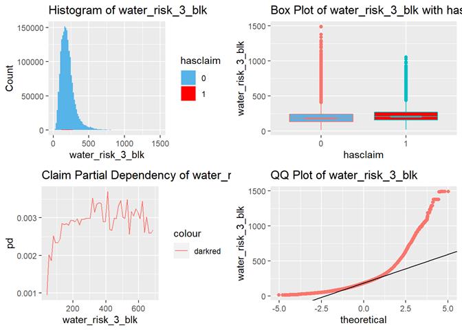
The higher the score, the more claims according to box-plots and partial dependency.
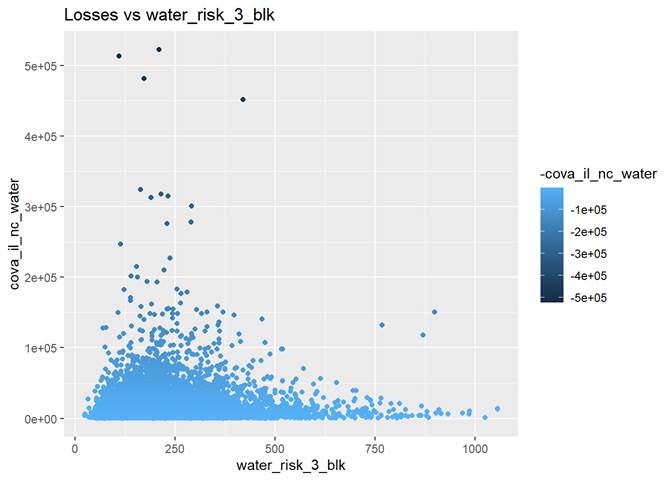
There are highest losses around 250 water_risk_3_blk.
water_risk_fre_3_blk
Non-weather Water Claim Frequency Index relative to Nation (0 to 5000: 100=average, 50=0.5x average, 500=5x average)
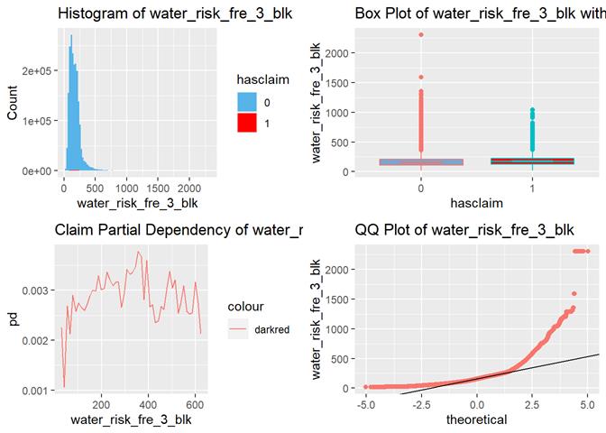
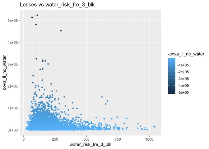
The highest losses are around 100
water_risk_sev_3_blk
Non-weather Water Claim Severity Index relative to Nation (0 to 5000: 100=average, 50=0.5x average, 500=5x average)
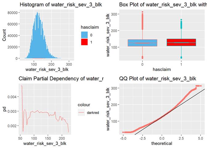
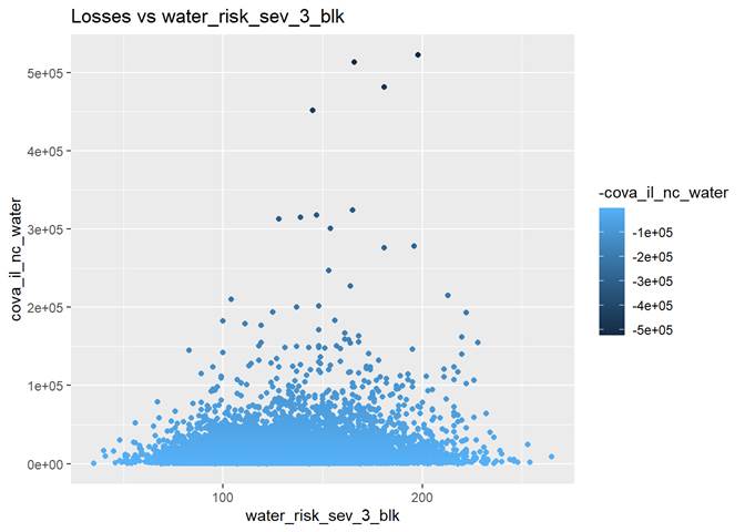
The highest losses are between 100 and 200 water_risk_sev_3_blk. We may have not enough data for higher numbers of water_risk_sev_3_blk
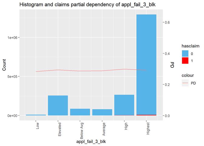
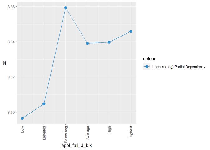
appl_fail_3_blk
Appliance failure rating
Cross Plot

Histogram and claims partial dependency
Baysian comparison
Losses mean plot with error bars
|
|
|
|
|
|
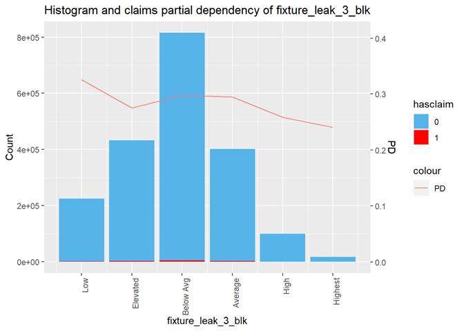
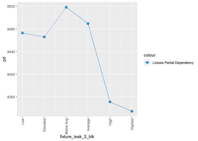
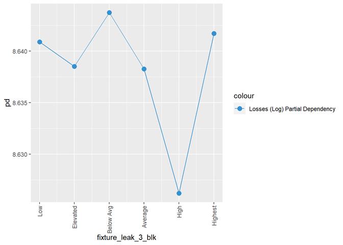
fixture_leak_3_blk
Fixture leak / overflow rating
Cross Plot

Histogram and claims partial dependency
Baysian comparison
Losses mean plot with error bars
|
|
|
|
|
|
pipe_froze_3_blk
Frozen pipe rating
Cross Plot

Histogram and claims partial dependency
Baysian comparison
Losses mean plot with error bars
|
|
|
|
|
|
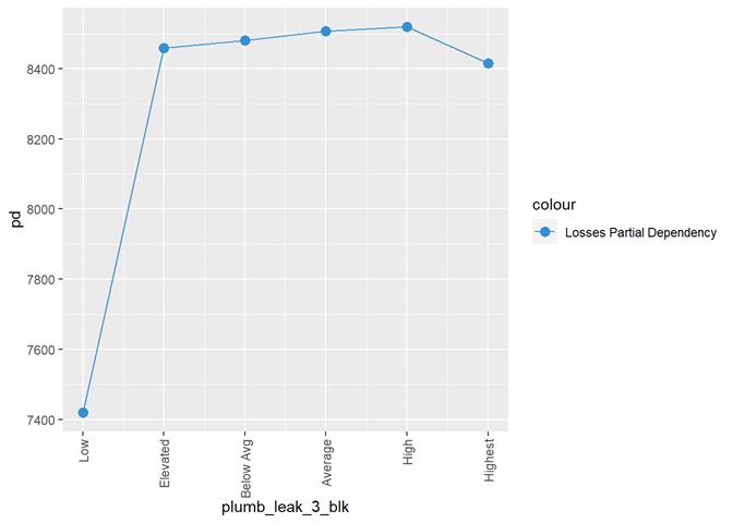
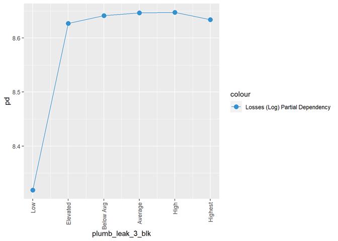
plumb_leak_3_blk
Plumbing
leak rating
Cross Plot
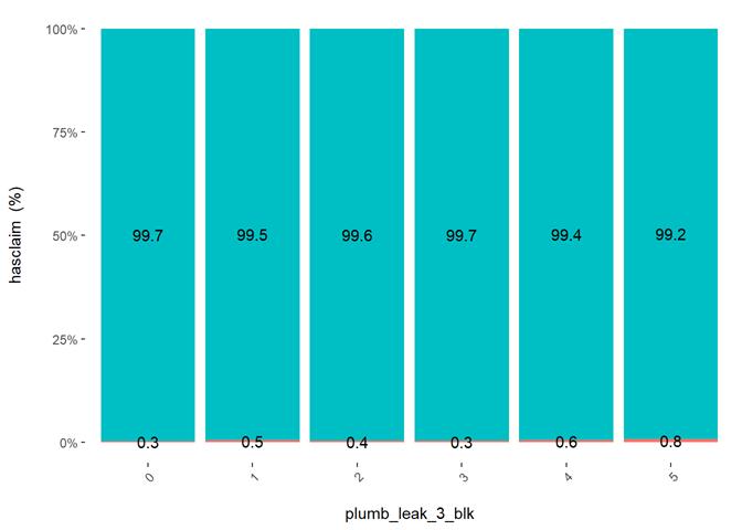
Histogram and claims partial dependency
Baysian comparison
Losses mean plot with error bars
|
|
|
|
|
|
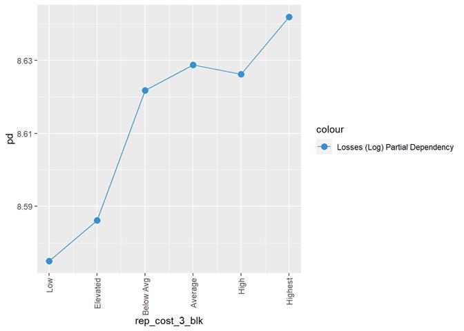
rep_cost_3_blk
Property
repair cost rating
Cross Plot

Histogram and claims partial dependency
Baysian comparison
Losses mean plot with error bars
|
|
|
|
|
|
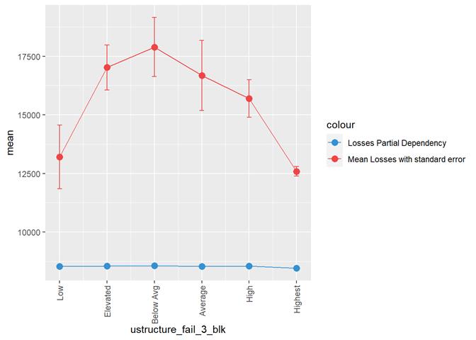
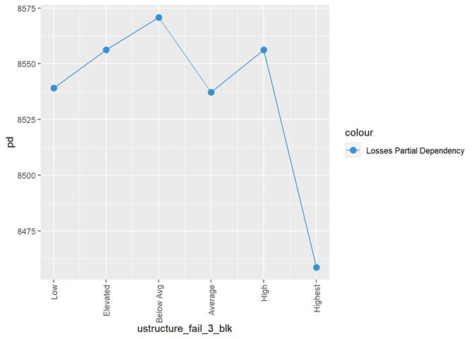
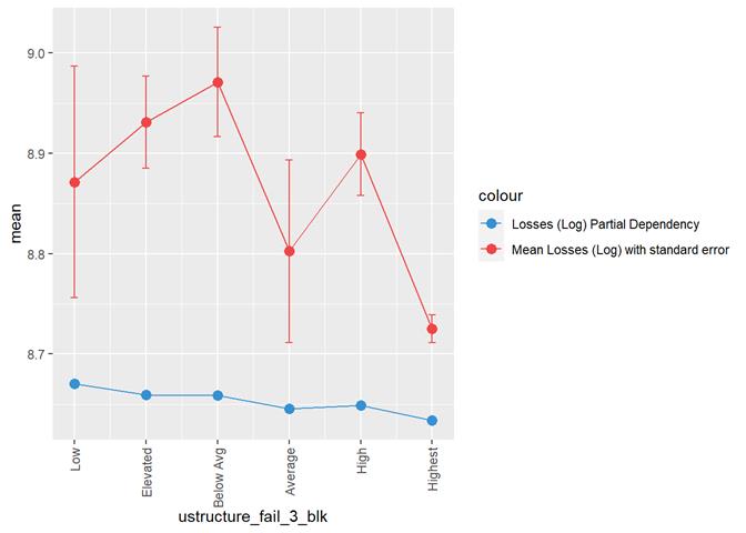
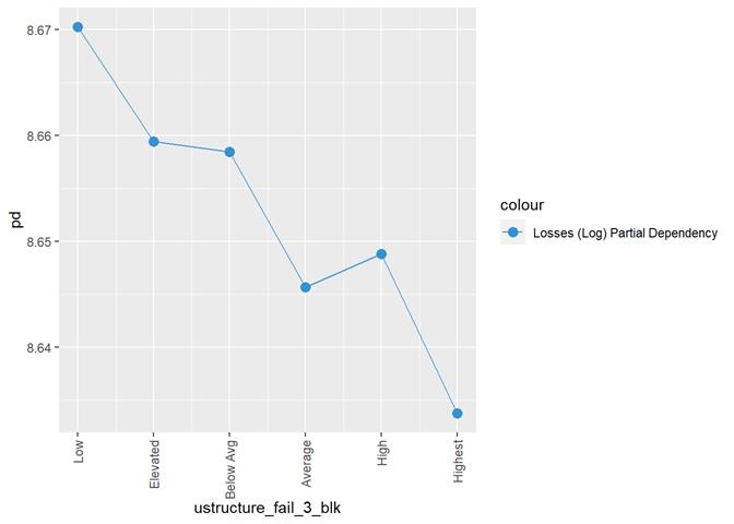
ustructure_fail_3_blk
Understructure
plumbing failure rating
Cross Plot

Histogram and claims partial dependency
Baysian comparison
Losses mean plot with error bars
|
|
|
|
|
|
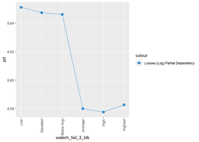
waterh_fail_3_blk
Water
heater failure rating
Cross Plot

Histogram and claims partial dependency
Baysian comparison
Losses mean plot with error bars
|
|
|
|
|
|
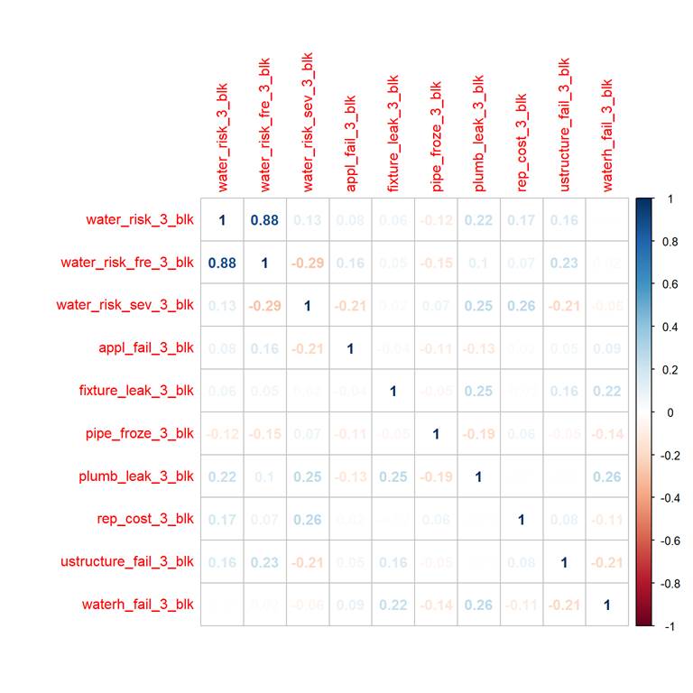
Correlation
R code and output:
There is a significant correlation between water_risk_3_blk and water_risk_fre_3_blk and some correlation between water_risk_fre_3_blk and water_risk_sev_3_blk.
And looks like water_risk_sev_3_blk is based on appl_fail_3_blk, plumb_leak_3_blk, rep_cost_3_blk and unstructured_fail_3_blk due to correlation.